Creativity on autopilot
While structure is entirely predictable, multiple structured notes gain an emergent property: Creativity. Let's look into how to setup our notes and generate novel ideas on autopilot.
My blog has moved
If you want to receive regular updates, new content and tips check out the website.
Creativity is connecting existing information in a novel way. Connect solutions to problems and you are creative.
This means that the more links we have, the easier this process becomes. But thinking how to connect a note to 100s of others is just infeasible.
In this post we will look into tags and maps of content (MOCs) to auto-connect notes without having to think of every connection.
MOCs and tags are an easy way to create 2-step connections. Obsidian’s graph feature will help us discover them.
Every novel 2-step connection will lead us to think of two “cousin” concepts we haven’t yet considered together. This is where innovation happens.
Examples:
Protein A and B are both involved in cell division → Do they interact, inhibit or enhance each other?
Algorithm A solves a singular value decomposition (SVD) task, Process B requires the SVD solution (i.e. Eigenvectors) to solve a problem. Can we integrate A to make B more efficient?
Remedy A alleviates a symptom B, symptom B occurs when we have iron deficiency. Is remedy A involved in the iron metabolism of the body?
Imagine that you have >100 of As and Bs in your notes (~10⁵ possible connections). Wouldn’t a system to discover those 2-step relations greatly increase the questions you ask and ideas you have?
It would – so let’s get started to create this system to become more creative.
1-step connections vs 2-step relations
Think of your notes as dots on a piece of paper. Every link in your note now connects it to another note. Many notes form a “graph” of notes.
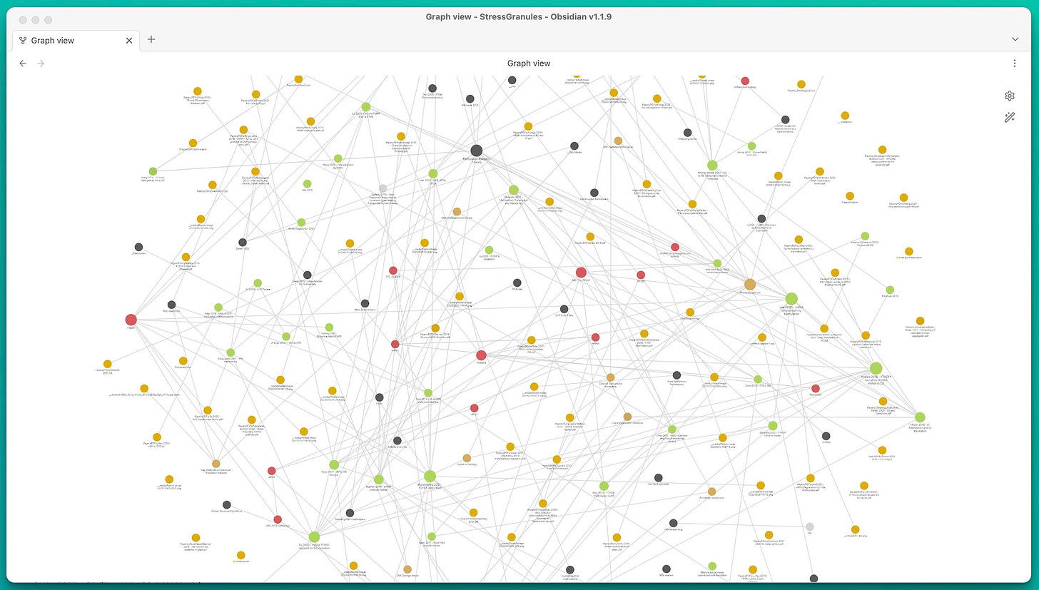
Too many notes form a mess - like this global graph of one of my (relatively small) vaults:
How many possible 1-step connections are there for N notes? If you mind the direction (i.e. A→B and B→A are different), you end up with N*(N - 1) possible connections. That is 9900 possible connections from just 100 notes.
You see - this quickly gets out of hand.
But: If you take good notes (see my 7 rules here), you link them at least to a few obvious partners.
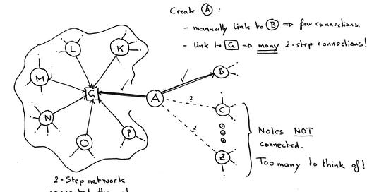
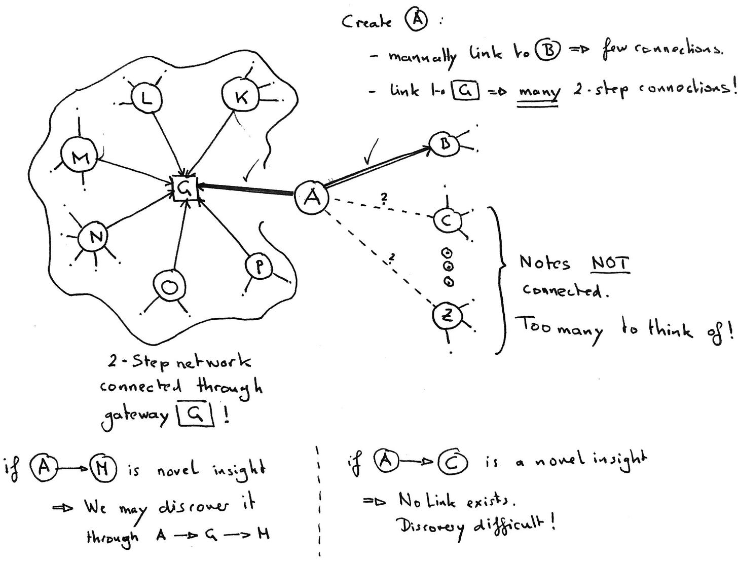
This forms a 2-step automatically by linking two notes to a shared partner: A→G and B→G. A and B are two steps away: A→G←B.
Let’s assume further that G is highly connected.
Linking our new note A→G thus connects it to a 2-step network. G acts as a gateway. And we effectively linked A to not only B but maybe dozens of other notes, yet we only thought of a single connection: A→G.
This mechanism is what we can use to amplify the number of connections made with every note.
1-step links: Need mental effort
2-step links: Can be automated as a consequence of linking to a gateway.
Tags and Maps of Content (MOCs) are exactly such a bridge - by looking at them through the graph we will discover these connections more readily.
Tags as links
Tags are labels that we can add to a note by just typing #tagA anywhere into the note. If you have never used them before, this is how it looks:
Obsidian is smart enough to recognize and remember the tags for you.
We often think of tags as a label to find or organize notes i.e. you can search for #tagA. But this is only one use of tags.
We can think of tags in a different way: as gateways.
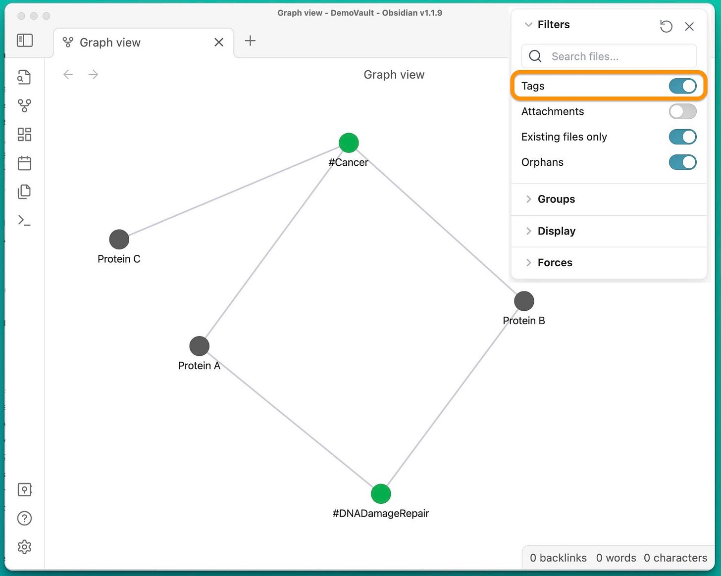
Obsidian’s graph feature (more below) allows us to do just this:
This simple graph has only 3 notes of hypothetic proteins. Notice that while A and B are not linked directly, they are related through the two tags #Cancer and #DNADamageRepair: A 2-step link.
It is only natural to start thinking about how A and B are connected in 1-step. Is one enhancing or inhibiting the other in a DNA damage repair pathway for example?
Important part here is that I discovered this question through the 2-step link, that was created by independently tagging A and B.
If you ask the right question (e.g. do A and B interact), you can potentially create a novel experiment and publish it. A new connection is a new publication.
How man tags to introduce?
Coming up with a system of tags is not always easy.
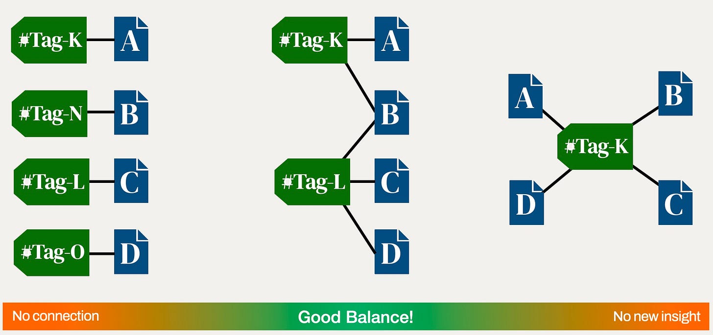
Too specific tags don’t connect well (worst case: each note has its own tag). Too generic tags connect too much (worst case: a single tag for all notes) and give no insight.
On the left we have “over engineering” on the right we have “lazyness”.
Finding a balance is key here.
(There is a constant debate in the personal knowledge management community whether and how to use tags or rely on searches. I say: A good craftsman never blames their tools.)
My strategy is to start with a few tags and break them down when you find that more than ~10-20 notes link to them. A straight forward way to do it are nested tags.
Example: Start with #protein after 10 proteins break it up into #protein/dnarepair, #protein/metabolism …
A nested tag is just a tag with a slash in it. It looks like “folders” in the tag menu.
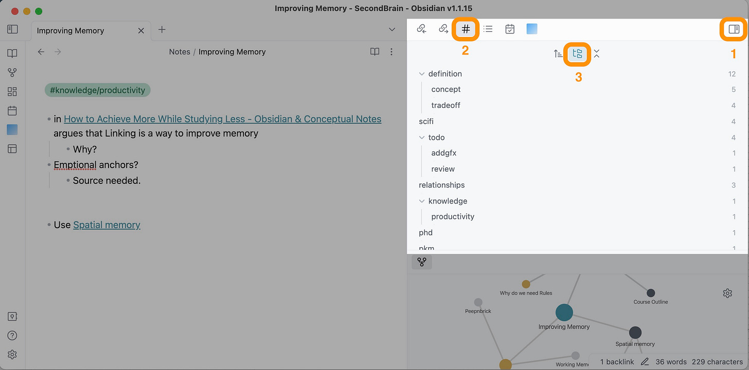
Here is how to use it: Open the sidebar (1), click on the tag menu (2) and select “show nested tags” (3). Now you can see the tags you are using and the number of notes in them. Seeing tags with too many notes → break them up into nested tags.
In this example, I had a tag #definition (to define something), but since it had 12 notes already, I broke it up into #definition/concept (to define a concept X) and #definition/tradeoff (a concept of type “X vs Y”).
Renaming or merging tags is something Obsidian does not do well out of the box. Luckily there is the Tag Wrangler plugin. Watch this short video in one of my tweets to learn how to use it. It can’t do much, but what it can do, saves us time.
Best practice: Explain your tagging
Add tags and explain why you added them. This will allow you to use the tag search more efficiently.
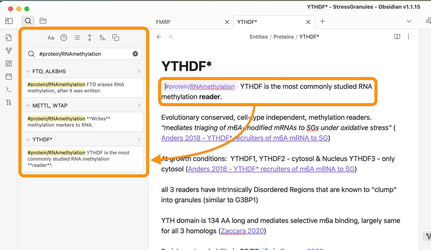
To do this type the tag and explanation into one paragraph. Here is how to use it:
Notice how the search for #protein/RNAmethylation gives me a little bit of context of how those proteins are involved in the complex mechanism of RNA methylation. While all of the proteins are involved in it, they have vastly different functions: reading, writing, or erasing methylation markers.
This one-sentence context will help greatly while searching complex topics.
(If I had many notes on methylation reader proteins, I might break it up into its own tag e.g. #protein/RNAMethylation/readers - but since there are only three notes, the context is a lot easier to use.)
The simpler tool that solves a problem is always the better tool (Occham’s razor variant).
Maps of Content (MOCs) as links
Maps of content are notes with the purpose of collecting links.
In the previous section, we added context to our tags. MOCs allow us to add even more context!
Naturally, you want to use MOCs when the nature of the connection is more complex.
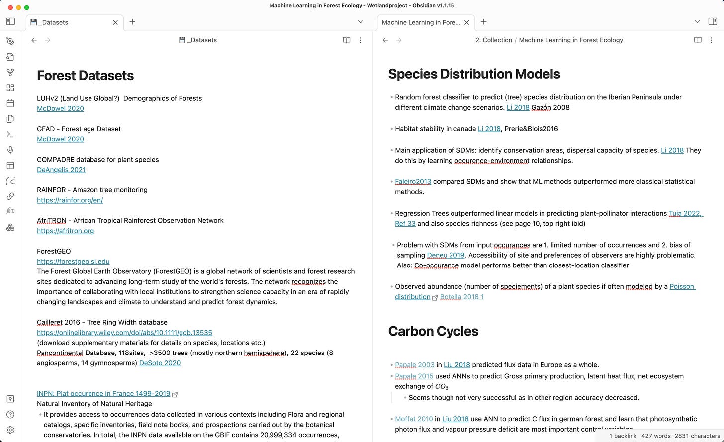
Two examples of context-heavy maps of content:
On the left, I collect datasets with forest data. As I want to develop an ecological forest model I might use these datasets to train and validate my model.
Some datasets are available upon request, so I link the paper that uses them. Others are online databases, so I add external links. The context describes what type of data it is.
On the right is a list of ecological models by function with a link to where they are used. Can you see already how well it prepares me to start writing an introduction chapter to a review paper titled “Machine learning applications in ecology”?
While I could tag the linked papers with “#machinelearning/SpeciesDistribution” to achieve the same effect, I would struggle to implement so much context.
Because applying a machine learning model to a problem is a process that can happen in infinite ways, its context is more complex. MOCs in this example are therefore a better solution than just some tags.
(In reality I use both. Two connections are stronger than one!)
More importantly: MOCs more prompt you to review information.
If you add to a MOC you will inevitably open and skim through it to find a place to add the new content. This process in itself gives me ideas sometimes.
The MOC acts as a gateway G and to connect our new note A we review all the other connections to G inside the MOCs. Effectively I review A→B, A→C … and maybe discover a new connection already.
In summary, MOCs provide more context than tags, but they take more time to maintain. They force you to review what you have written and provide a great resource to start introduction chapters!
Discovery using the Obsidian graph view
We have now two ways to auto-connect notes: Maps of Content (MOCs) and tags. How do we go about discovering these novel 2-step connections?
The graph will give us this insight.
There are two types of graphs: Local and Global. An example of the global graph is the big tangly mess (image at the beginning of this post). It is in my opinion relatively useless.
Local graphs
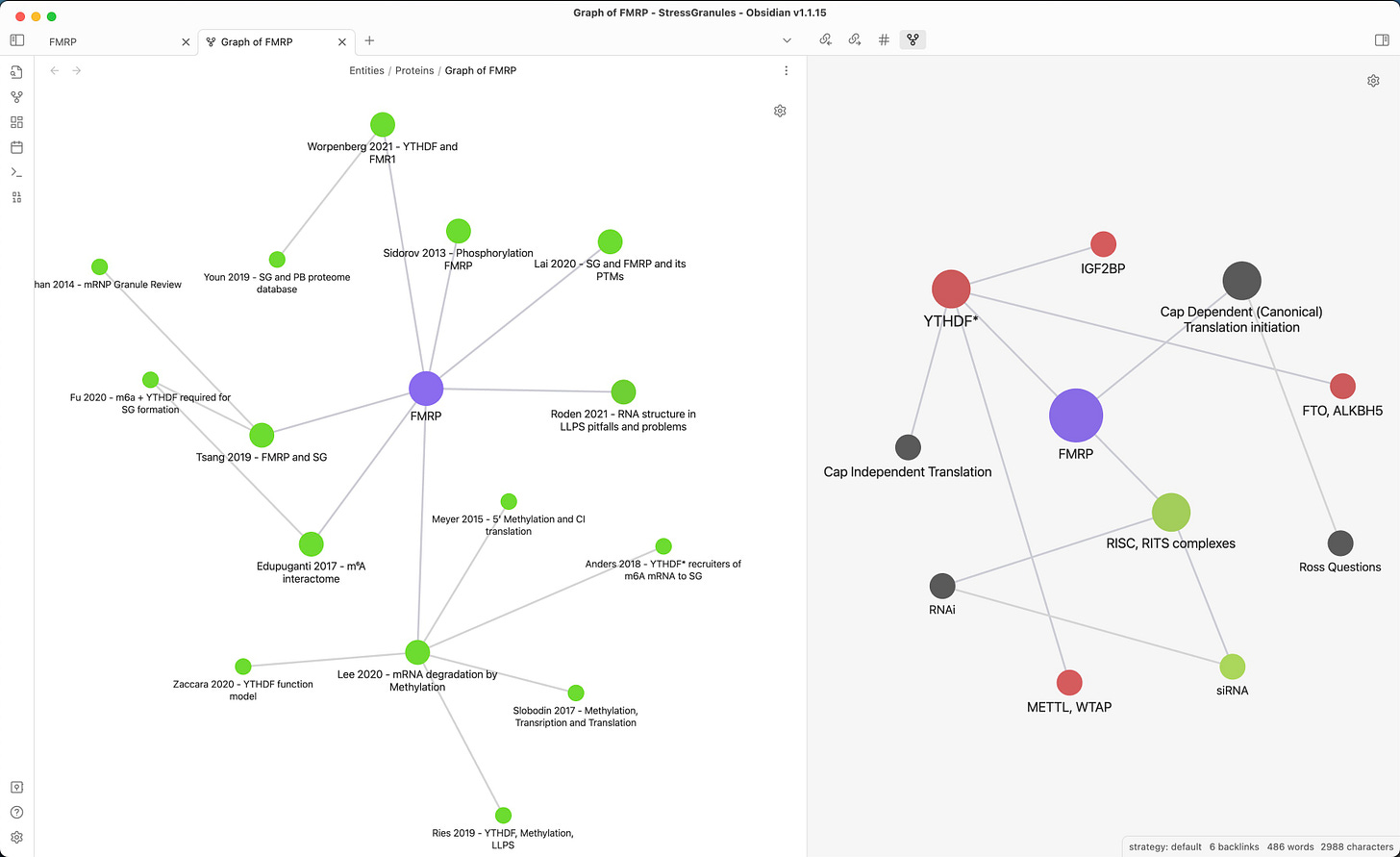
Local graphs on the other hand only show the neighbourhood of a note. Here is an example of the FMRP protein:
On the left, I filter the graph to only show publications mentioning this protein and their connections. We could call it “Publication graph”.
On the right, I filter it to display other proteins (red), non-proteins (green), and other things (gray). We could call it “Interaction graph”.
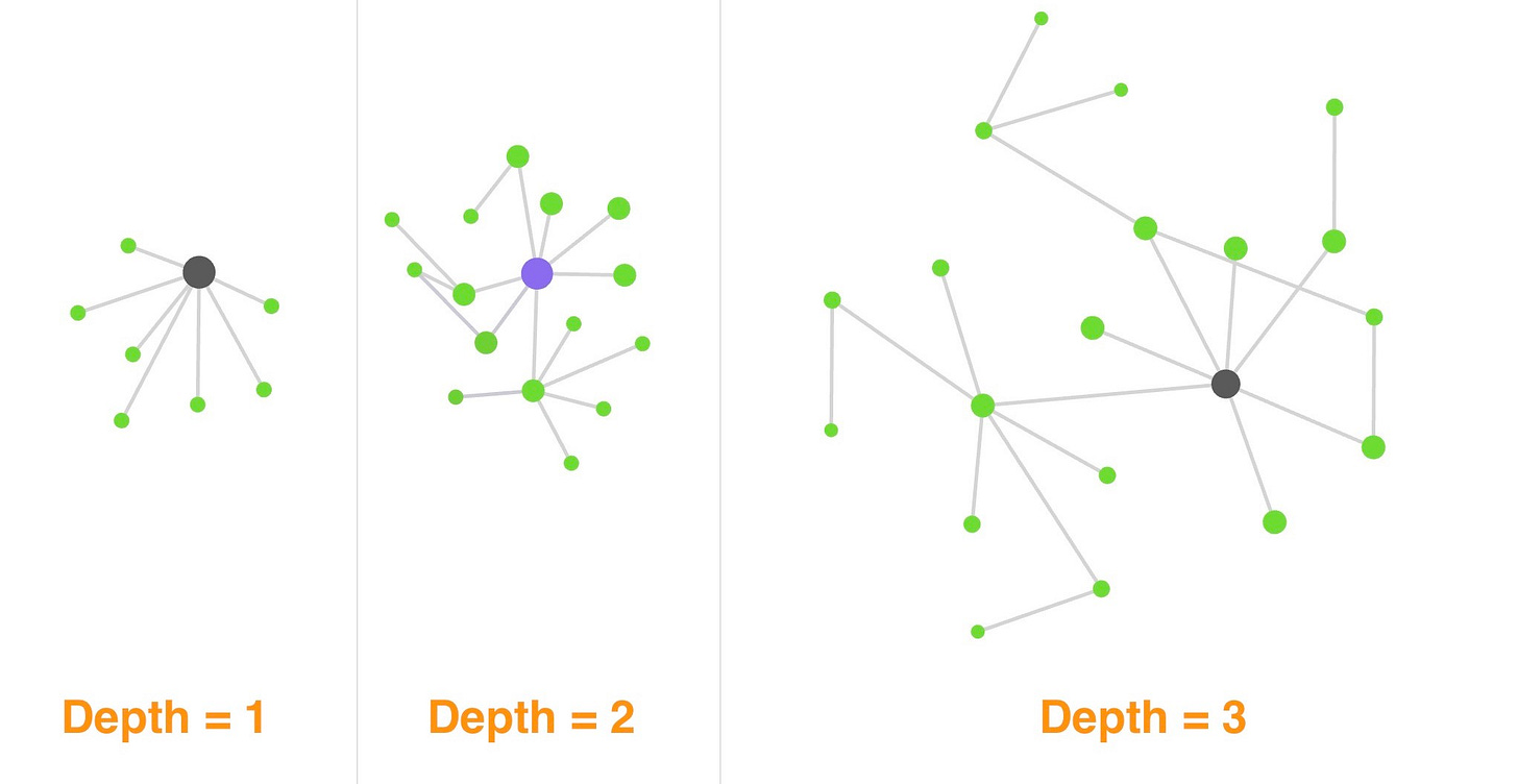
The number of notes a local graph displays is controlled by its depth. The depth is the number of steps I step away from my current note:
Graphs are useful only if you don’t have too many nodes. Set the depth to ≥ 2 as this is when you will start discovering novel connections.
How to configure local graphs
This feature is only accessible through the command palette. Hit cmd or ctrl + P, in the popup menu type in “local graph” and open the feature. Configuring the graph is as everything in Obsidian reduced to the essentials. I made a good tutorial on Twitter about this:

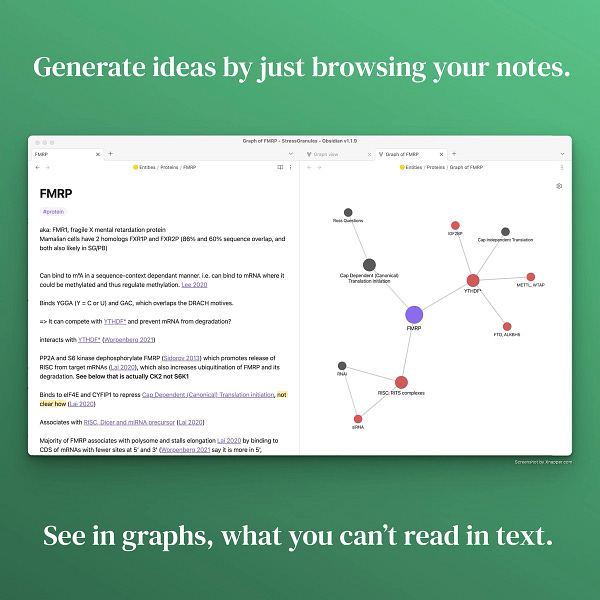
Since in this article we more focus on the theory of why to use the graphs, I will refer you to this tweet to learn how to setup filters and define colors (there are many pictures in the tweet).
You can have as many graphs as you need and place them into sidebars, tabs or separate windows. Depending on how much space you have on your desktop you can set them up differently.
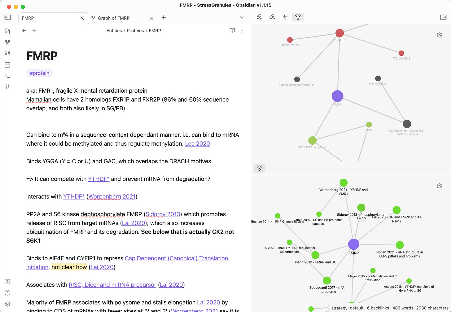
Here is my preference on my 15” laptop:
Both graphs are in the right sidebar and I can collapse or expand them with a hotkey.
The top graph shows interaction partners, which make more sense for proteins. Therefore it sits next to the tag tab and can be switched for tags (which is useful in all notes).
The bottom graph are related papers, which is useful to almost every note in my vault, so I keep it visible when the sidebar is visible - even if the tags tab is open.
Tags and MOCs in the graph
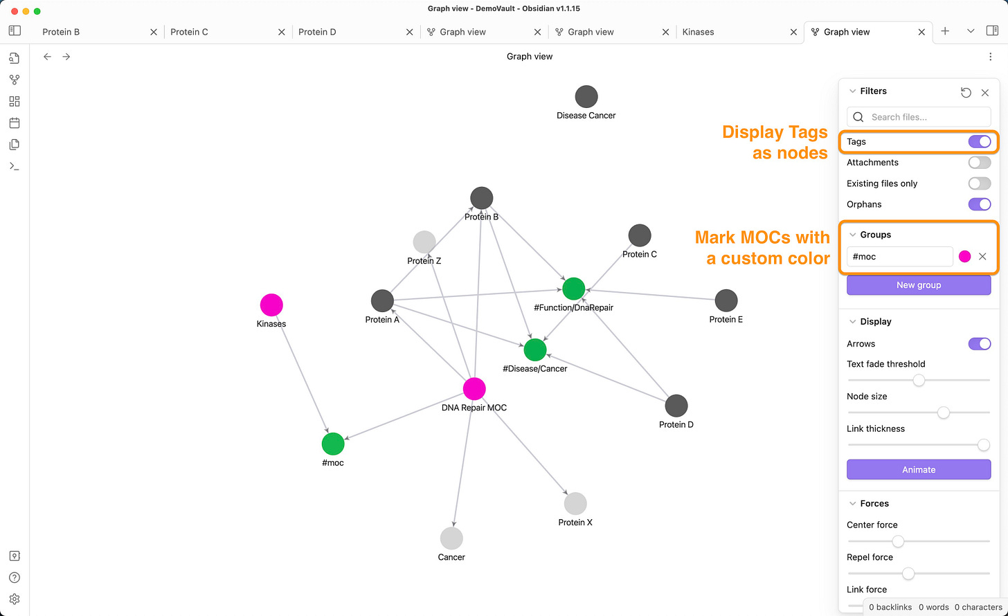
To show tags in your graph, activate the tags checkbox under “filters” and you will see your tags displayed as notes.
To show MOCs in your graph you need to create a filter. You can think of a specific tag like #moc for all your MOCs. Configure a “group” that will identify all MOCs and give them a color.
Doing both at the same time might be a bit of an overload. But I hope it gives you an idea how to use the graph creatively.
Discovery
If you have ever been foraging for mushrooms in the forest or sea shells on the beach you know there is no secret to finding things. You just have to look over and over again in the right place.
The right place here is our setup: multiple local graphs for multiple aspects of our notes (e.g. interaction partners, publications). Set them up for your domain and they will provide a good hunting ground for new ideas.
Some examples:
A historian might have have a type of note “People” and for any event (e.g. birth of christ) have a graph displaying the connections (e.g. Virgin Mary, Joseph). They might discover how people’s “friends/connections” might have influenced a historic event.
An agriculturist might have a type of notes for the chemical requirements of a specific tree (i.e. moist, nitrogen rich soils) and practices that create these conditions (i.e. mulching for moisture and green manure for nitrogen fertilization). She might discover that combining a lesser known agriculture practice will enhance a specific crop in a way no one thought of.
Graphs won’t work out of the box. (Just like the first beach you go to won’t be perfect for finding the most beautiful sea shells).
Think what type of graph will likely give you insight. Configure it and use for a while to find out what works and what doesn’t.
Obsidian allows you to save layouts for your tabs/sidebars into a “workspace”, this way you can store your configurations and switch between them. It is a core plugin, but deactivated by default. Go to settings > core plugins > workspaces to activate it. Experiment with different layouts and find what feels right!
Summary
Introducing tags and maps of content (MOCs) connects notes through 2-step links.
You don’t need to think of every possible connection but only of the connection from note to tag or MOC. Each of these connects you to the tag’s or MOC’s network.
Then you can use a local graph to discover meaningful 2-step connections. This will not happen by itself, but through smart configuration of the local graph i.e. filtering for a subset of notes, setting the depth to 2 and color coding the nodes.
We can create multiple graphs for different aspects. Store them out of the way in the sidebar to not clutter your note space.
As you browse and re-read your notes, you can now pay attention to your graph to discover 2-step connections as you go.
Need help with literature discovery?
In Gourmet Literature Review I introduced how I used litmaps to discover, prioritize and structure the literature review process. Having tested a few tools since, I am still very happy with litmaps. It is luxurious, powerful and fun to use.
Try it out and if you like it use the code EffortlessAcademic in the checkout to get a 10% discount.

